Habitat-species associations
Given a number of tree species and habitat types in a plot, are species significantly aggregated within habitats?
Mauro Lepore
2020-12-05
Source:vignettes/siteonly/tt_test.Rmd
tt_test.RmdThis article shows how to determine habitat-species associations with the function tt_test(), developed by Sabrina Russo, Daniel Zuleta, Matteo Detto, and Kyle Harms.
Setup
First, install and load (“open”) the relevant packages.
# install.packages("remotes")
remotes::install_github("forestgeo/fgeo")
library(dplyr)
#>
#> Attaching package: 'dplyr'
#> The following objects are masked from 'package:stats':
#>
#>     filter, lag
#> The following objects are masked from 'package:base':
#>
#>     intersect, setdiff, setequal, union
library(ggplot2)
library(fgeo.x)
library(fgeo.tool)
#>
#> Attaching package: 'fgeo.tool'
#> The following object is masked from 'package:stats':
#>
#>     filter
library(fgeo.analyze)
# For reproducible results
set.seed(1014)
Load census and habitat data
We will use example datasets that come with fgeo.analyze.
census <- fgeo.x::download_data("luquillo_tree6_random")

str(census)
#> tibble [1,000 × 19] (S3: tbl_df/tbl/data.frame)
#>  $ treeID   : int [1:1000] 104 119 180 602 631 647 1086 1144 1168 1380 ...
#>  $ stemID   : int [1:1000] 143 158 225 736 775 793 1339 1410 1438 1702 ...
#>  $ tag      : chr [1:1000] "10009" "100104" "100171" "100649" ...
#>  $ StemTag  : chr [1:1000] "10009" "100104" "100174" "100649" ...
#>  $ sp       : chr [1:1000] "DACEXC" "MYRSPL" "CASARB" "GUAGUI" ...
#>  $ quadrat  : chr [1:1000] "113" "1021" "921" "821" ...
#>  $ gx       : num [1:1000] 10.3 182.9 164.6 149 38.3 ...
#>  $ gy       : num [1:1000] 245 410 410 414 245 ...
#>  $ MeasureID: int [1:1000] 582850 578696 617049 614253 598429 614211 603131 616923 603151 614023 ...
#>  $ CensusID : int [1:1000] 6 6 6 6 6 6 6 6 6 6 ...
#>  $ dbh      : num [1:1000] 195 44.9 46.1 33.1 139 248 176 75 613 NA ...
#>  $ pom      : chr [1:1000] "1.45" "1.25" "1.35" "1.3" ...
#>  $ hom      : num [1:1000] 1.45 1.26 1.34 1.3 1.25 1.35 1.42 1.3 1.25 NA ...
#>  $ ExactDate: Date[1:1000], format: "2016-04-20" "2016-08-04" ...
#>  $ DFstatus : chr [1:1000] "alive" "alive" "alive" "alive" ...
#>  $ codes    : chr [1:1000] "MAIN;A" "MAIN;A" "SPROUT;A" "MAIN;A" ...
#>  $ nostems  : num [1:1000] 1 1 2 1 1 1 1 1 1 1 ...
#>  $ status   : chr [1:1000] "A" "A" "A" "A" ...
#>  $ date     : num [1:1000] 20564 20670 20670 20664 20565 ...
# Creating habitat data from elevation data
elevation <- fgeo.x::elevation
habitat <- fgeo_habitat(elevation, gridsize = 20, n = 4)
str(habitat)
#> tibble [400 × 3] (S3: fgeo_habitat/fgeo_topography/tbl_df/tbl/data.frame)
#>  $ gx      : num [1:400] 0 0 0 0 0 0 0 0 0 0 ...
#>  $ gy      : num [1:400] 0 20 40 60 80 100 120 140 160 180 ...
#>  $ habitats: int [1:400] 1 1 1 1 1 1 1 1 1 1 ...
fgeo.plot::autoplot(habitat)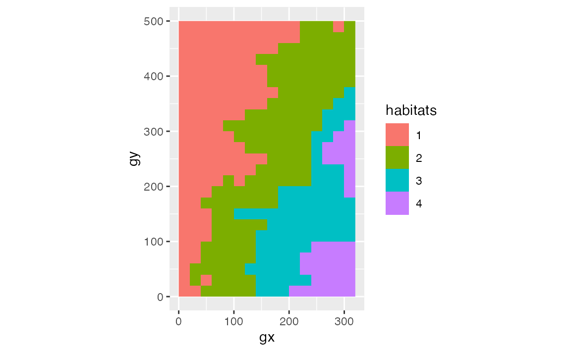
To load your own data, you may run something like this:
Pick data
We will pick alive trees, of 10 mm or more, and of sufficiently abundant species.
pick <- filter(
  census,
  # Keep only alive
  status == "A",
  # Keep dbh of 10 mm or more (drops missing dbh)
  dbh >= 10
)
# Count number of rows per species
pick <- add_count(pick, sp)
# Keep sufficiently abundant trees
pick <- filter(pick, n > 50)

# Summary
unique(select(pick, sp, n))
#> # A tibble: 3 x 2
#>   sp         n
#>   <chr>  <int>
#> 1 CASARB    66
#> 2 PREMON   234
#> 3 SLOBER    66
Overview
Before testing, we can overview the relationship between species and habitats with a plot.
# Tweaks
offset <- 20 / 2
habitat2 <- mutate(
  habitat,
  # Center species and habitat data
  x = gx + offset,
  y = gy + offset,
  # From continuous to categorical
  habitats = as.factor(habitats)
)
ggplot(pick, aes(x = gx, y = gy)) +
  geom_raster(data = habitat2, aes(x, y, fill = habitats)) +
  geom_point() +
  coord_fixed() +
  facet_wrap(~sp) +
  labs(fill = "Habitat")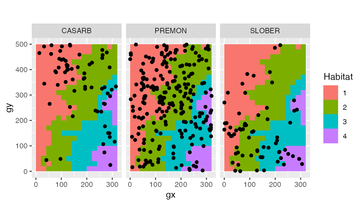
tt_test() and any number of species
tt_test_result <- tt_test(pick, habitat)
#> Using `plotdim = c(320, 500)`. To change this value see `?tt_test()`.
#> Using `gridsize = 20`. To change this value see `?tt_test()`.
#> Warning: Is `census` a tree table (not a stem table)? See `?tt_test()`.
tt_test_result
#> [[1]]
#>        N.Hab.1 Gr.Hab.1 Ls.Hab.1 Eq.Hab.1 Rep.Agg.Neut.1 Obs.Quantile.1 N.Hab.2
#> CASARB      29     1242      356        2              0          0.776      20
#>        Gr.Hab.2 Ls.Hab.2 Eq.Hab.2 Rep.Agg.Neut.2 Obs.Quantile.2 N.Hab.3
#> CASARB      390     1206        4              0          0.244      12
#>        Gr.Hab.3 Ls.Hab.3 Eq.Hab.3 Rep.Agg.Neut.3 Obs.Quantile.3 N.Hab.4
#> CASARB      778      817        5              0          0.486       5
#>        Gr.Hab.4 Ls.Hab.4 Eq.Hab.4 Rep.Agg.Neut.4 Obs.Quantile.4
#> CASARB      932      658       10              0          0.583
#>
#> [[2]]
#>        N.Hab.1 Gr.Hab.1 Ls.Hab.1 Eq.Hab.1 Rep.Agg.Neut.1 Obs.Quantile.1 N.Hab.2
#> PREMON      91     1093      504        3              0          0.683      89
#>        Gr.Hab.2 Ls.Hab.2 Eq.Hab.2 Rep.Agg.Neut.2 Obs.Quantile.2 N.Hab.3
#> PREMON     1254      344        2              0          0.784      40
#>        Gr.Hab.3 Ls.Hab.3 Eq.Hab.3 Rep.Agg.Neut.3 Obs.Quantile.3 N.Hab.4
#> PREMON      305     1292        3              0          0.191      14
#>        Gr.Hab.4 Ls.Hab.4 Eq.Hab.4 Rep.Agg.Neut.4 Obs.Quantile.4
#> PREMON      270     1322        8              0          0.169
#>
#> [[3]]
#>        N.Hab.1 Gr.Hab.1 Ls.Hab.1 Eq.Hab.1 Rep.Agg.Neut.1 Obs.Quantile.1 N.Hab.2
#> SLOBER      18      273     1324        3              0          0.171      24
#>        Gr.Hab.2 Ls.Hab.2 Eq.Hab.2 Rep.Agg.Neut.2 Obs.Quantile.2 N.Hab.3
#> SLOBER      810      788        2              0          0.506      17
#>        Gr.Hab.3 Ls.Hab.3 Eq.Hab.3 Rep.Agg.Neut.3 Obs.Quantile.3 N.Hab.4
#> SLOBER     1155      440        5              0          0.722       7
#>        Gr.Hab.4 Ls.Hab.4 Eq.Hab.4 Rep.Agg.Neut.4 Obs.Quantile.4
#> SLOBER     1292      303        5              0          0.807
To help you interpret the results, you can use summary().
summary(tt_test_result)
#> # A tibble: 12 x 3
#>    sp     habitat association
#>    <chr>  <chr>   <chr>
#>  1 CASARB 1       neutral
#>  2 CASARB 2       neutral
#>  3 CASARB 3       neutral
#>  4 CASARB 4       neutral
#>  5 PREMON 1       neutral
#>  6 PREMON 2       neutral
#>  7 PREMON 3       neutral
#>  8 PREMON 4       neutral
#>  9 SLOBER 1       neutral
#> 10 SLOBER 2       neutral
#> 11 SLOBER 3       neutral
#> 12 SLOBER 4       neutral
You may want to combine the output into a single matrix by row-binding each element of the results-list.
Reduce(rbind, tt_test_result)
#>        N.Hab.1 Gr.Hab.1 Ls.Hab.1 Eq.Hab.1 Rep.Agg.Neut.1 Obs.Quantile.1 N.Hab.2
#> CASARB      29     1242      356        2              0          0.776      20
#> PREMON      91     1093      504        3              0          0.683      89
#> SLOBER      18      273     1324        3              0          0.171      24
#>        Gr.Hab.2 Ls.Hab.2 Eq.Hab.2 Rep.Agg.Neut.2 Obs.Quantile.2 N.Hab.3
#> CASARB      390     1206        4              0          0.244      12
#> PREMON     1254      344        2              0          0.784      40
#> SLOBER      810      788        2              0          0.506      17
#>        Gr.Hab.3 Ls.Hab.3 Eq.Hab.3 Rep.Agg.Neut.3 Obs.Quantile.3 N.Hab.4
#> CASARB      778      817        5              0          0.486       5
#> PREMON      305     1292        3              0          0.191      14
#> SLOBER     1155      440        5              0          0.722       7
#>        Gr.Hab.4 Ls.Hab.4 Eq.Hab.4 Rep.Agg.Neut.4 Obs.Quantile.4
#> CASARB      932      658       10              0          0.583
#> PREMON      270     1322        8              0          0.169
#> SLOBER     1292      303        5              0          0.807
You also can gather all results into a single dataframe – this lets you use a wide range of tools for data manipulation and visualization.
as_tibble(tt_test_result)
#> # A tibble: 12 x 8
#>    habitat sp     N.Hab Gr.Hab Ls.Hab Eq.Hab Rep.Agg.Neut Obs.Quantile
#>  * <chr>   <chr>  <dbl>  <dbl>  <dbl>  <dbl>        <dbl>        <dbl>
#>  1 1       CASARB    29   1242    356      2            0        0.776
#>  2 2       CASARB    20    390   1206      4            0        0.244
#>  3 3       CASARB    12    778    817      5            0        0.486
#>  4 4       CASARB     5    932    658     10            0        0.583
#>  5 1       PREMON    91   1093    504      3            0        0.683
#>  6 2       PREMON    89   1254    344      2            0        0.784
#>  7 3       PREMON    40    305   1292      3            0        0.191
#>  8 4       PREMON    14    270   1322      8            0        0.169
#>  9 1       SLOBER    18    273   1324      3            0        0.171
#> 10 2       SLOBER    24    810    788      2            0        0.506
#> 11 3       SLOBER    17   1155    440      5            0        0.722
#> 12 4       SLOBER     7   1292    303      5            0        0.807
You can benefit from storing your results in a dataframe. Compared to a matrix, a dataframe fits better in common workflows for data manipulation and visualization. The dataframe is the most important data structure used in dplyr, ggplot2, and many other packages. Here are some examples of what you can do with our dataframe output. (The next few code chunks use the pipe operator (%>%) to avoid saving intermediary results and to make our code more expressive – where each line is an imperative statement that communicates our intention.)
- Pick interesting rows and sort them in a meaningful way.
as_tibble(tt_test_result) %>%
  filter(sp == "CASARB")
#> # A tibble: 4 x 8
#>   habitat sp     N.Hab Gr.Hab Ls.Hab Eq.Hab Rep.Agg.Neut Obs.Quantile
#>   <chr>   <chr>  <dbl>  <dbl>  <dbl>  <dbl>        <dbl>        <dbl>
#> 1 1       CASARB    29   1242    356      2            0        0.776
#> 2 2       CASARB    20    390   1206      4            0        0.244
#> 3 3       CASARB    12    778    817      5            0        0.486
#> 4 4 CASARB 5 932 658 10 0 0.583- Summarize
as_tibble(tt_test_result) %>%
  group_by(sp, habitat) %>%
  summarize(total_stem_count = sum(N.Hab))
#> `summarise()` regrouping output by 'sp' (override with `.groups` argument)
#> # A tibble: 12 x 3
#> # Groups:   sp [3]
#>    sp     habitat total_stem_count
#>    <chr>  <chr>              <dbl>
#>  1 CASARB 1                     29
#>  2 CASARB 2                     20
#>  3 CASARB 3                     12
#>  4 CASARB 4                      5
#>  5 PREMON 1                     91
#>  6 PREMON 2                     89
#>  7 PREMON 3                     40
#>  8 PREMON 4                     14
#>  9 SLOBER 1                     18
#> 10 SLOBER 2                     24
#> 11 SLOBER 3                     17
#> 12 SLOBER 4                      7