 Analyze forest diversity and dynamics
fgeo helps you to install, load, and access the documentation of multiple packages to analyze forest diversity and dynamics (fgeo.analyze, fgeo.plot, fgeo.tool, fgeo.x). This package-collection allows you to manipulate and plot ForestGEO data, and to do common analyses including abundance, demography, and species-habitats associations.
Installation
Make sure your R environment is as follows:
- R version is recent
- All packages are updated (run
update.packages(); maybe useask = FALSE) - No other R session is running
- Current R session is clean (click Session > Restart R)
Install the latest stable version of fgeo from CRAN with:
Or install the development version of fgeo from GitHub with:
Example
library(fgeo)
#> ── Attaching packages ────────────────────────────────────────── fgeo 1.1.3.9000 ──
#> ✔ fgeo.analyze 1.1.10.9000     ✔ fgeo.tool    1.2.5
#> ✔ fgeo.plot    1.1.8           ✔ fgeo.x       1.1.4
#> ── Conflicts ────────────────────────────────────────────────── fgeo_conflicts() ──
#> ✖ fgeo.tool::filter() masks stats::filter()
Explore fgeo
On an interactive session, fgeo_help() and fgeo_browse_reference() help you to search documentation.
Access and manipulate data
example_path() allows you to access datasets stored in your R libraries.
example_path()
#>  [1] "csv"           "mixed_files"   "rdata"         "rdata_one"
#>  [5] "rds"           "taxa.csv"      "tsv"           "vft_4quad.csv"
#>  [9] "view"          "weird"         "xl"

(vft_file <- example_path("view/vft_4quad.csv"))
#> [1] "/home/mauro/R/x86_64-pc-linux-gnu-library/3.6/fgeo.x/extdata/view/vft_4quad.csv"
read_<table>()
read_vft() and read_taxa() import a ViewFullTable and ViewTaxonomy from .tsv or .csv files.
read_vft(vft_file)
#> # A tibble: 500 x 32
#>     DBHID PlotName PlotID Family Genus SpeciesName Mnemonic Subspecies
#>     <int> <chr>     <int> <chr>  <chr> <chr>       <chr>    <chr>
#>  1 385164 luquillo      1 Rubia… Psyc… brachiata   PSYBRA   <NA>
#>  2 385261 luquillo      1 Urtic… Cecr… schreberia… CECSCH   <NA>
#>  3 384600 luquillo      1 Rubia… Psyc… brachiata   PSYBRA   <NA>
#>  4 608789 luquillo      1 Rubia… Psyc… berteroana  PSYBER   <NA>
#>  5 388579 luquillo      1 Areca… Pres… acuminata   PREMON   <NA>
#>  6 384626 luquillo      1 Arali… Sche… morototoni  SCHMOR   <NA>
#>  7 410958 luquillo      1 Rubia… Psyc… brachiata   PSYBRA   <NA>
#>  8 385102 luquillo      1 Piper… Piper glabrescens PIPGLA   <NA>
#>  9 353163 luquillo      1 Areca… Pres… acuminata   PREMON   <NA>
#> 10 481018 luquillo      1 Salic… Case… arborea     CASARB   <NA>
#> # … with 490 more rows, and 24 more variables: SpeciesID <int>,
#> #   SubspeciesID <chr>, QuadratName <chr>, QuadratID <int>, PX <dbl>,
#> #   PY <dbl>, QX <dbl>, QY <dbl>, TreeID <int>, Tag <chr>, StemID <int>,
#> #   StemNumber <int>, StemTag <int>, PrimaryStem <chr>, CensusID <int>,
#> #   PlotCensusNumber <int>, DBH <dbl>, HOM <dbl>, ExactDate <date>,
#> #   Date <int>, ListOfTSM <chr>, HighHOM <int>, LargeStem <chr>,
#> #   Status <chr>
pick_<what>() and drop_<what>()
fgeo is pipe-friendly. You may not use pipes but often they make code easier to read.
Use %>% to emphasize a sequence of actions, rather than the object that the actions are being performed on.
– https://style.tidyverse.org/pipes.html
pick_dbh_under(), drop_status() and friends pick and drop rows from a ForestGEO ViewFullTable or census table.
(census <- fgeo.x::tree5)
#> # A tibble: 30 x 19
#>    treeID stemID tag   StemTag sp    quadrat    gx    gy MeasureID CensusID
#>     <int>  <int> <chr> <chr>   <chr> <chr>   <dbl> <dbl>     <int>    <int>
#>  1   7624 160987 1089… 175325  TRIP… 722     139.  425.     486675        5
#>  2   8055  10036 1094… 109482  CECS… 522      94.8 424.     468874        5
#>  3  19930 117849 1234… 165576  CASA… 425      61.3 496.     471979        5
#>  4  23746  29677 14473 14473   PREM… 617     100.  328.     442571        5
#>  5  31702  39793 22889 22889   SLOB… 304      53.8  73.8    447307        5
#>  6  35355  44026 27538 27538   SLOB… 1106    203.  110.     449169        5
#>  7  35891  44634 282   282     DACE… 901     172.   14.7    434266        5
#>  8  39705  48888 33371 33370   CASS… 1010    184.  194.     451067        5
#>  9  50184  60798 5830  5830    MATD… 1007    191.  132.     437645        5
#> 10  57380 155867 66962 171649  SLOB… 1414    274.  279.     459427        5
#> # … with 20 more rows, and 9 more variables: dbh <dbl>, pom <chr>,
#> #   hom <dbl>, ExactDate <date>, DFstatus <chr>, codes <chr>,
#> #   nostems <dbl>, status <chr>, date <dbl>

census %>%
  pick_dbh_under(100)
#> # A tibble: 18 x 19
#>    treeID stemID tag   StemTag sp    quadrat    gx    gy MeasureID CensusID
#>     <int>  <int> <chr> <chr>   <chr> <chr>   <dbl> <dbl>     <int>    <int>
#>  1   7624 160987 1089… 175325  TRIP… 722     139.  425.     486675        5
#>  2  19930 117849 1234… 165576  CASA… 425      61.3 496.     471979        5
#>  3  31702  39793 22889 22889   SLOB… 304      53.8  73.8    447307        5
#>  4  35355  44026 27538 27538   SLOB… 1106    203.  110.     449169        5
#>  5  39705  48888 33371 33370   CASS… 1010    184.  194.     451067        5
#>  6  57380 155867 66962 171649  SLOB… 1414    274.  279.     459427        5
#>  7  95656 129113 1315… 131519  OCOL… 402      79.7  22.8    474157        5
#>  8  96051 129565 1323… 132348  HIRR… 1403    278    40.6    474523        5
#>  9  96963 130553 1347… 134707  TETB… 610     114.  182.     475236        5
#> 10 115310 150789 1652… 165286  MANB… 225      24.0 497.     483175        5
#> 11 121424 158579 1707… 170701  CASS… 811     146.  218.     484785        5
#> 12 121689 158871 1712… 171277  INGL… 515      84.2 285.     485077        5
#> 13 121953 159139 1718… 171809  PSYB… 1318    247.  354.     485345        5
#> 14 124522 162698 1742… 174224  CASS… 1411    279.  210.     488386        5
#> 15 125038 163236 1753… 175335  CASS… 822     153.  426.     488924        5
#> 16 126087     NA 1773… <NA>    CASA… 521      89.8 408.         NA       NA
#> 17 126803     NA 1785… <NA>    PSYB… 622     113.  426          NA       NA
#> 18 126934     NA 1787… <NA>    MICR… 324      47   480.         NA       NA
#> # … with 9 more variables: dbh <dbl>, pom <chr>, hom <dbl>,
#> #   ExactDate <date>, DFstatus <chr>, codes <chr>, nostems <dbl>,
#> #   status <chr>, date <dbl>
pick_main_stem() and pick_main_stemid() pick the main stem or main stemid(s) of each tree in each census.
add_<column(s)>()
add_status_tree()adds the column status_tree based on the status of all stems of each tree.
stem %>%
  select(CensusID, treeID, stemID, status) %>%
  add_status_tree()
#> # A tibble: 1,320 x 5
#>    CensusID treeID stemID status status_tree
#>       <int>  <int>  <int> <chr>  <chr>
#>  1        6    104    143 A      A
#>  2        6    119    158 A      A
#>  3       NA    180    222 G      A
#>  4       NA    180    223 G      A
#>  5        6    180    224 G      A
#>  6        6    180    225 A      A
#>  7        6    602    736 A      A
#>  8        6    631    775 A      A
#>  9        6    647    793 A      A
#> 10        6   1086   1339 A      A
#> # … with 1,310 more rows
add_index() and friends add columns to a ForestGEO-like dataframe.
stem %>%
  select(gx, gy) %>%
  add_index()
#> Guessing: plotdim = c(320, 500)
#> * If guess is wrong, provide the correct argument `plotdim`
#> # A tibble: 1,320 x 3
#>       gx    gy index
#>    <dbl> <dbl> <dbl>
#>  1  10.3  245.    13
#>  2 183.   410.   246
#>  3 165.   410.   221
#>  4 165.   410.   221
#>  5 165.   410.   221
#>  6 165.   410.   221
#>  7 149.   414.   196
#>  8  38.3  245.    38
#>  9 143.   411.   196
#> 10  68.9  253.    88
#> # … with 1,310 more rows
Plot data
For simplicity, we will focus on only a few species.
autoplot() and friends produce different output depending on the class of input. You can create different input classes, for example, with sp() and sp_elev():
- Use
sp(census)to plot the columnspof acensusdataset – i.e. to plot species distribution.
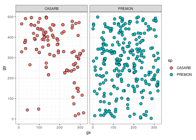
- Use
sp_elev(census, elevation)to plot the columnsspandelevof acensusandelevationdataset, respectively – i.e. to plot species distribution and topography.
elevation <- fgeo.x::elevation
class(sp_elev(stem_2sp, elevation))
#> [1] "sp_elev" "list"

autoplot(sp_elev(stem_2sp, elevation))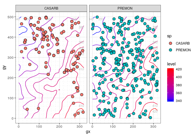
Analyze
Abundance
abundance() and basal_area() calculate abundance and basal area, optionally by groups.
abundance(
  pick_main_stem(census)
)
#> # A tibble: 1 x 1
#>       n
#>   <int>
#> 1    30

by_species <- group_by(census, sp)

basal_area(by_species)
#> # A tibble: 18 x 2
#> # Groups:   sp [18]
#>    sp     basal_area
#>    <chr>       <dbl>
#>  1 CASARB      437.
#>  2 CASSYL     4146.
#>  3 CECSCH   144150.
#>  4 DACEXC    56832.
#>  5 GUAGUI     9161.
#>  6 HIRRUG      131.
#>  7 INGLAU      141.
#>  8 MANBID      167.
#>  9 MATDOM    45239.
#> 10 MICRAC        0
#> 11 OCOLEU      437.
#> 12 PREMON    78864.
#> 13 PSYBER        0
#> 14 PSYBRA      154.
#> 15 SCHMOR    41187.
#> 16 SLOBER    23377.
#> 17 TETBAL      272.
#> 18 TRIPAL       93.3
Demography
recruitment_ctfs(), mortality_ctfs(), and growth_ctfs() calculate recruitment, mortality, and growth. They all output a list. as_tibble() converts the output from a list to a more convenient dataframe.
tree5 <- fgeo.x::tree5

as_tibble(
  mortality_ctfs(tree5, tree6)
)
#> Detected dbh ranges:
#>   * `census1` = 10.9-323.
#>   * `census2` = 10.5-347.
#> Using dbh `mindbh = 0` and above.
#> # A tibble: 1 x 9
#>       N     D    rate   lower  upper  time  date1  date2 dbhmean
#>   <dbl> <dbl>   <dbl>   <dbl>  <dbl> <dbl>  <dbl>  <dbl>   <dbl>
#> 1    27     1 0.00834 0.00195 0.0448  4.52 18938. 20590.    101.
Species-habitats association
tt_test() runs a torus translation test to determine habitat associations of tree species. as_tibble() converts the output from a list to a more convenient dataframe. summary() helps you to interpret the result.
# This analysis makes sense only for tree tables
tree <- download_data("luquillo_tree5_random")

habitat <- fgeo.x::habitat
result <- tt_test(tree, habitat)
#> Using `plotdim = c(320, 500)`. To change this value see `?tt_test()`.
#> Using `gridsize = 20`. To change this value see `?tt_test()`.

as_tibble(result)
#> # A tibble: 292 x 8
#>    habitat sp     N.Hab Gr.Hab Ls.Hab Eq.Hab Rep.Agg.Neut Obs.Quantile
#>  * <chr>   <chr>  <dbl>  <dbl>  <dbl>  <dbl>        <dbl>        <dbl>
#>  1 1       ALCFLO     2   1443    153      4            0        0.902
#>  2 2       ALCFLO     1    807    778     15            0        0.504
#>  3 3       ALCFLO     0      0    715    885           -1        0
#>  4 4       ALCFLO     0      0    402   1198           -1        0
#>  5 1       ALCLAT     0      0    544   1056           -1        0
#>  6 2       ALCLAT     1   1432    156     12            0        0.895
#>  7 3       ALCLAT     0      0    324   1276           -1        0
#>  8 4       ALCLAT     0      0    144   1456           -1        0
#>  9 1       ANDINE     1   1117    466     17            0        0.698
#> 10 2       ANDINE     1   1081    510      9            0        0.676
#> # … with 282 more rows

summary(result)
#> # A tibble: 292 x 3
#>    sp     habitat association
#>    <chr>  <chr>   <chr>
#>  1 ALCFLO 1       neutral
#>  2 ALCFLO 2       neutral
#>  3 ALCFLO 3       repelled
#>  4 ALCFLO 4       repelled
#>  5 ALCLAT 1       repelled
#>  6 ALCLAT 2       neutral
#>  7 ALCLAT 3       repelled
#>  8 ALCLAT 4       repelled
#>  9 ANDINE 1       neutral
#> 10 ANDINE 2       neutral
#> # … with 282 more rows
R code from recent publications by ForestGEO partners
Data have been made available as required by the journal to enable reproduction of the results presented in the paper. Please do not share these data without permission of the ForestGEO plot Principal Investigators (PIs). If you wish to publish papers based on these data, you are also required to get permission from the PIs of the corresponding ForestGEO plots.
- Soil drivers of local-scale tree growth in a lowland tropical forest (Zemunik et al., 2018).
-
Plant diversity increases with the strength of negative density dependence at the global scale (LaManna et al., 2018)
- Response #1: LaManna et al. 2018. Response to Comment on “Plant diversity increases with the strength of negative density dependence at the global scale” Science Vol. 360, Issue 6391, eaar3824. DOI: 10.1126/science.aar3824
- Response #2: LaManna et al. 2018. Response to Comment on “Plant diversity increases with the strength of negative density dependence at the global scale”. Science Vol. 360, Issue 6391, eaar5245. DOI: 10.1126/science.aar5245
Acknowledgments
Thanks to all partners of ForestGEO for sharing their ideas and code. For feedback on fgeo, special thanks to Gabriel Arellano, Stuart Davies, Lauren Krizel, Sean McMahon, and Haley Overstreet. For all other help, I thank contributors in the the documentation of the features they helped with.
